ITA Baranov’s Walkthrough. Chapter 2

19 Dec 2016

Insertion Sort

Chapter 2 introduces insertion sort, an algorithm that solves the sorting problem mentioned in a previous chapter.

Input: A sequence of n numbers <a₁, a₂, …, a_n>
Output: A permutation <b₁, b₂, …, b_n> of the input sequence such that b₁ ≤ b₂ ≤ … ≤ b_n

INSERTION-SORT(A)						cost 	times
for j = 2 to A.length						c₁	n
	key = A[j]						c₂	n-1
	// Insert A[j] into the sorted sequence A[1..j-1].	0	n-1
	i = j - 1						c₄	n-1	
	while i > 0 and A[i] > key				c₅	Σ(j=2 to n) t_j
	  A[i+1] = A[i]						c₆	Σ(j=2 to n) t_j - 1
	  i = i - 1						c₇	Σ(j=2 to n) t_j - 1
	A[i+1] = key						c₈	n-1

Basically, algorithm divides the sequence in two parts. The left part A[1…j-1] constitutes the currently sorted subarray and the right part is a subarray A[j+1…n] that corresponds to the numbers to be sorted. What you want to do is to pick an element (starting from 2), go down the array and try to find a good spot to fit the number in, at the same time copying the values one place over to have a free slot for insertion.

Analyzing algorithms

Running Time T(N): The running time of the algorithm is the sum of running times for each statement executed; a statement that takes c_i steps to execute and executes n times will contribute c_in to the total running time.

T(N) = c₁*n c₂(n-1) +c₄(n-1) +c₅Σj +c₆Σ(t_j-1) +c₇Σ(t_j-1) +c₈(n-1).

Algorithm’s running time does depend on the input. For example, if the input array is sorted, we would have A[i] key when i has its initial value of j-1. Thus t_j = 1 for j = 2, 3 … n and the T(N) would be:
T(N) = c₁n +c₂(n-1) +c₄(n-1) +c₅(n-1) +c₈(n-1) = (c₁+..c₈)n - (c₂+c₄+c₅+c₈) = Cn - c
This clearly looks like a linear function of n.

Another example, array is in reverse sorted order, then we must compare the entire left subarray which would make t_j = j for j = 2, 3 … n. Consequently, T(N) would look like:
T(N) = c₁n +c₂(n-1) +c₄(n-1) +c₅(n(n+1)/2-1) + c₆(n(n-1)/2) + c₇(n(n-1)/2) +c₈(n-1)
= Cn² + Cn - c
This clearly looks like a quadratic function of n.

Notice that Σ(j=2 to n)[j] = n(n+1)/2-1 and Σ(j=2 to n)[j-1] = n(n-1)/2

When we try to analyze algorithms, we usually only care about finding the worst-case running times. Why?

It gives an upper bound on the running time for any input. Knowing it provides a guarantee that the algorithm will never take any longer.
In some cases, worst case occurs fairly often (e.g. searching a database for non-existent information)
The “average case” is often roughly as bad as the worst case. For example, imagine that half of the elements in A[1…j-1] are less than A[j] and half are greater. It would make t_j = j/2 which would be the same quadratic formula but divided by a constant (2), not a huge difference.

To denote the worst case we write the running time of Θ(n²) (pronounced “theta of n-squared”) which represents a rate of growth or order of growth. We can ignore the lower-order terms because they are relatively insignificant for large values of n. All we care about is the leading term of the formula (e.g., cn²).

Algorithm Design & Mergesort

Sometimes, we can come up with a different approach to tackle the same problem. So far we used an incremental approach: to sort the subarray A[1…j-1], we inserted a single element A[j] into its proper place, yielding the sorted subarray. A different way of doing things would be using divide-and-conquer method: break the problem into several subproblems that are similar to the original problem but smaller in size, solve the subproblems recursively, and finally combine these solutions to create a solution to the original problem. Mergesort algorithm would be a good example of this.

Divide: Divide the n-element sequence to be sorted into two subsequences of n/2 elements each.
Conquer: Sort the two subsequences recursively using merge sort.
Combine: Merge the two sorted subsequences to produce a fully sorted sequence.

The following MERGE function merges two sorted subarrays A[p..q] and A[q + 1..r] where p ≤ q ≤ r. It merges them to form a single sorted subarray that replaces the current subarray A[p..r]. Since we perform at most n steps, where each step is just a comparing of two elements from left and right subarrays, merging takes Θ(N) time.

MERGE(A,p,q,r)
n1 = q-p+1
n2 = r-q
let L[1..n1+1] and R[1..n2 +1] be new arrays
for i = 1 to n1
	L[i] = A[p+i-1]
for j=1 to n2
	R[j] = A[q+j]
L[n1+1] = inf
L[n2+1] = inf
i = 1
j = 1
for k = p to r
	if L[i] <= R[j]
		A[k] = L[i]
		i = i + 1
	else A[k] = R[j]
		j = j + 1

Compute the length of A[p..q] and A[q+1..r].
Create left and right of lengths n₁+1 and n₂+1. Extra position holds the sentinel which would simplify our code.
For loops copy the subarray A[p..q] into L[1..n₁] and A[q+1..r] into R[1..n₂].
Put the sentinels.
Put the values in A in order.

Now we can use merge procedure as a subroutine in the merge sort algorithm. The procedure sorts the elements in the subarray A[p..r]. If p ≥ r the subarray has at most one element and is therefore already sorted. Otherwise, the divide step simply computes an index q that partitions A[p..r] into two subarrays: A[p..q], containing ceil(n/2) elements and A[q+1..r], containing floor(n/2) elements.

MERGE-SORT(A,p,r)
if p < r
	q = floor((p+r)/2)
	MERGE-SORT(A,p,q)
	MERGE-SORT(A,q+1,r)
	MERGE(A,p,q,r)

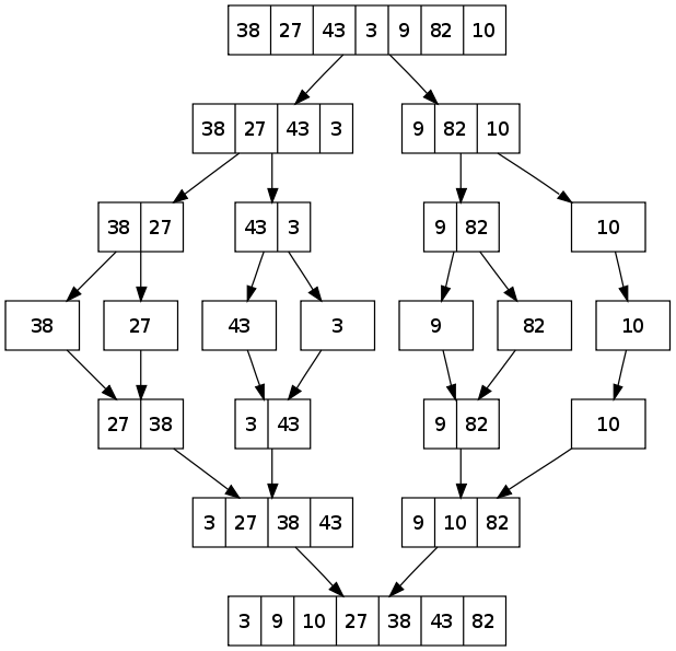
To sort an entire array, we make the initial call MERGE-SORT(A,1,A.length). The algorithms goes all the way to the bottom, merges pairs of 1-item seqs to form sorted seqs of length 2, merges pairs of seqs of length 2 to form sorted seqs of length 4 and so on, until two sequences of length n/2 are merged to form the final sorted sequence of length n.

image-center

Runtime Complexity

T(n) is either going to be Θ(1) if n ≤ c or aT(n/b) + D(n) + C(n).
In our case:
1) D(n) is Θ(1) operation (finding q) [Divide]
2) We recursively solve two subproblems, each of size n/2, which contributes to 2T(n/2) to the running time [Conquer]
3) We have seen that MERGE takes Θ(N) time on n-element subarray so C(N) = Θ(N) [Combine]
Thus, we get T(n) = Θ(1) [if n ≤ c] or 2T*(n/2) + Θ(n) [if n > 1]

So what exactly is 2T*(n/2)? To find it out, let’s refer to a recursion tree to better understand the first term.

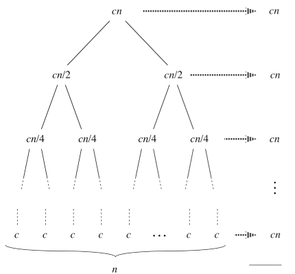
Recursion Tree: A recursion tree is useful for visualizing what happens when a recurrence is iterated. It diagrams the tree of recursive calls and the amount of work done at each call.

image-center

First level takes cn time.
Second level takes 2(cn/2) = cn.
Third level takes 4(cn/4) = cn.
To find out the total running time we need to sum up all the costs on each level. How do we know the number of levels?

Number of levels of the recursion tree: The total number of levels of the recursion tree is lgn + 1, where n is the number of leaves, corresponding to the input size.

Then, our recursion tree has lgn + 1 levels, each costing cn, for a total of cn(lgn + 1) = cnlgn + cn.
Substitute this in our previous T(n) equation and we get:
T(n) = Θ(1) [if n ≤ c] or cnlgn + cn + Θ(n) = Θ(nlgn) [if n > 1].
This is a much better runtime complexity than the insertion sort we looked at earlier.

Twitter Facebook Google+