The maximum-subarray problem
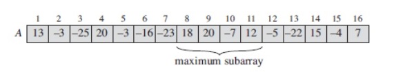
The maximum subarray problem is the task of finding the contiguous subarray within a one-dimensional array of numbers which has the largest sum. The trick is that the numbers can be negative, otherwise it would be too easy. Let’s think how can we approach this problem using divide-and-conquer technique. Probably, we should divide the array in two parts, left and right. Then our maximum subarray must either be:
1) entirely in the subarray A[low..mid], so that low ≤ i ≤ j ≤ mid,
2) entirely in the subarray A[mid+1..high], so that mid ≤ i ≤ j ≤ high, or
3) crossing the midpoint, so that low ≤ i ≤ mid < j ≤ high
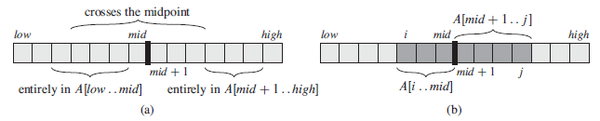
Since the last part would not really be a smaller instance of our original problem, because it has the added restriction that the subarray it chooses must cross the midpoint, we should consider it to be in the combine part of our divide-and-conquer technique. All we need to do is to find 4.4(b) maximum subarrays of the form A[i..mid] and A[mid+1..j] and then combine them together.
FIND-MAX-CROSSING-SUBARRAY(A,low,mid,high)
left-sum = -inf
sum = 0
for i = mid downto low
	sum = sum + A[i]
	if sum > left-sum
		left-sum = sum
		max-left = i
right-sum = -inf
sum = 0
for j = mid + 1 to high
	sum = sum + A[j]
	if sum > right-sum
		right-sum = sum
		max-right = j
return (max-left,max-right,left-sum + right-sum);
If the subarray A[low..high] contains n entries (so that n = high - low + 1), the call FIND-MAX-CROSSING-SUBARRAY(A,low,mid,high) takes Θ(n) time. Since each iteration of each of the two for loops takes Θ(1) time, we just need to count up how many iterations there are altogether. We have:
(left) + (right) = (mid - low + 1) + (high - mid) = high - low + 1 = n
Now we are ready to start writing our divide-and-conquer algorithm to solve the problem:
FIND-MAXIMUM-SUBARRAY(A,low,high)
if high==low [Base Case: only one element]
	return (low,high,A[low])
else
	mid = floor((low+high)/2)
	(left-low,left-high,left-sum) =
		FIND-MAXIMUM-SUBARRAY(A,low,mid)
	(right-low,right-high,right-sum) =
		FIND-MAXIMUM-SUBARRAY(A,mid+1,high)
	(cross-low,cross-high,cross-sum) =
		FIND-MAX-CROSSING-SUBARRAY(A,low,mid,high)
	if left-sum >= right-sum and left-sum >= cross-sum
		return (left-low,left-high,left-sum)
	elseif right-sum >= left-sum and right-sum >= cross-sum
		return (right-low, right-high, right-sum)
	else return (cross-low, cross-high,cross-sum)
Let’s setup a recurrence that describes the running time of this function:
T(n): Θ(1) + 2T(n/2) + Θ(n) + Θ(1) = 2T(n/2) + Θ(n).
Since it looks the same as the recurrence for the merge-sort algorithm discussed in Chapter 2, we know that the solution should be T(n) = Θ(nlgn);
Recurrences
Recurrences go hand in hand with the divide-and conquer paradigm discussed in Chapter 2, because they give us a natural way to characterize the running times of such algorithms. For example, we could have a recursive algorithm that divides subproblems into unequal sizes, such as a 2/3-to-1/3 split. If the divide and combine steps take linear time, such an algorithm would give rise to the recurrence T(n) = T(2n/3) + T(n/3) + Θ(n).
There are three methods for solving recurrences (obtaining asymptotic Θ or O bounds on the solution):
In the substitution method, we guess a bound and then use mathematical induction to prove our guess correct.
The recursion-tree method converts the recurrence into a tree whose nodes represent the costs incurred at various levels of the recursion.
The master method provides bounds for recurrences of the form T(n) = aT(n/b) + f(n) - where algorithm creates subproblems, each of which is n/b the size of the original problem, and in which the divide and combine steps together take f(n) time.
The substitution method for solving recurrences
For example, T(n) = 2T(floor(n/2)) + n. We may guess that the solution is T(n) = O(nlgn) since it reminds us about the recurrence we’ve seen earlier. The substitution method requires us to prove that T(n) ≤ cnlgn for an appropriate choice of the constant c > 0.We start by assuming that this bound holds for all positive number m < n, in particular for m = (floor(n/2)), yielding T((floor(n/2)) ≤ c(floor(n/2))lg(floor(n/2)). Substitute this into recurrence and we get:
T(n)
≤ 2(c(floor(n/2))lg(floor(n/2))) + n
≤ cnlg(n/2) + n
= cnlgn - cnlg2 + n
= cnlgn - cn + n ≤ cnlgn
An easy way to avoid a second step would be to pick a c that makes this inequality come true for sufficiently large n. As we can see, it holds if c ≥ 1. However, a right way to do it is to use mathematical induction to prove base and inductive steps, which I am not going to talk through since we would make this chapter even broader.
The recursion-tree method for solving recurrences
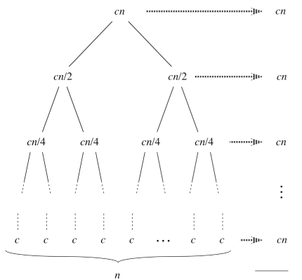
We have already seen this method in Chapter 2 when we tried to derive the running time for the merge-sort algorithm. There are few things to remember:
The subproblem decrease by a factor of a each time we go down one level, we eventually must reach a boundary condition. How far from the root do we reach one? The subproblem for a node at depth i is n/ai. This, the subproblem size hits n = 1 when n/ai = 1 or when i = logan. Thus, the tree has logan + 1 levels.
What’s the cost at each level of the tree? Each level has b times more nodes that the level above, and so the number of nodes at depth i is bi. Since subproblem sizes reduce by a factor of a for each level we go down from the root, each node at depth i, has a cost of F(n/ai). Multiplying this by the number of nodes at each level we get bi*F(n/ai). The bottom level, at depth logan, has b(logan) = n(logab) each contributing cost T(1).
The master method for solving recurrences
Let A ≥ 1 and b > 1 be constants, let f(n) be a function, and let T(n) be defined on the nonnegative integers by the recurrence
T(n) = aT(n/b) + f(n). Then T(n) has the following asymptotic bounds:
If f(n) = O(nlogba-e) for some constant e > 0, then T(n) = Θ(nlogba)
If f(n) = Θ(nlogba), then T(n) = Θ(nlogba * lgn)
If f(n) = Ω(nlogba+e) for some constant e > 0, and if af(n/b) ≤ cf(n) for some constant c less than 1 and all sufficiently large n, then T(n) = Θ(f(n))
In each of three cases, we compare the function f(n) with the function (nlogba). The largest of the two would be the solution to the recurrence.
Important note: in order to use rule 1 f(n) must be polynomially smaller than (nlogba) [polynomially larger for rule 3]
Examples:
T(n) = 9T(n/3) + n
a = 9, b = 3, f(n) = n, and thus we have (nlogba) = Θ(n2). Since f(n) = O((nlog39-e), where e = 1, we can apply case 1 of the master theorem and conclude that the solution is T(n) = Θ(n2). An easier way to remember this might be to take the power of f(n), let’s say d, and check the relationship between a and bd. [9 > 31 -> case 1]
T(n) = T(2n/3) + 1
(nlogba) = 1. Case 2 applies, since f(n) = Θ(nlogba) = Θ(1), and thus the solution to the recurrence is T(n) = Θ(lgn) [1 = 3/20 = 1 -> case 2]
T(n) = 3T(n/4) + nlgn
(nlogba) = O(n0.793). Since f(n) = Ω(nlog43+e), where e ~ 0.2, case 3 applies if we can show that the regularity condition holds for f(n). For sufficiently large n, we have that af(n/b) = 3(n/4)lg(n/4) ≤ (3/4) nlgn = cf(n) for c = 3/4. Thus, T(n) = Θ(nlgn). [3 < 4log43 = 40.793 = 0.30021 -> case 3]