Quicksort
The quicksort algorithm has a worst-case running time of Θ(n2) on an input array of n numbers. Despite this slow worst-case running time, quicksort is often the best practical choice for sorting because it is remarkably efficient on the average: its expected running time is Θ(nlgn), and the constant factors hidden in the Θ(nlgn) notation are quite small. It also has the advantage of sorting in place and it works well even in virtual-memory environments.
Description of quicksort
Quicksort, like merge sort, applies the divide-and-conquer paradigm introduced in Chapter 2:
Divide: Partition (rearrange) the array A[p..r] into two (possibly empty) subarrays A[p..q-1] and A[q+1..r] such that each element of A[p..q-1] less than or equal to A[q], which is, in turn, less than or equal to each element of A[q+1..r]. Compute the index q as part of this partitioning procedure.
Conquer: Sort the two subarrays A[p..q-1] and A[q+1..r] by recursive call to quicksort.
Combine: Because the subarrays are already sorted, no work is needed to combine them: the entire array A[p..r] is now sorted.
QUICKSORT(A,p,r)
if p < r
	q = PARTITION(A,p,r)
	QUICKSORT(A,p,q-1)
	QUICKSORT(A,q+1,r)
Partitioning the array
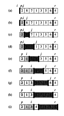
The key to the algorithm is the PARTITION procedure, which rearranges the subarray A[p..r] in place:
PARTITION(A,p,r)
x = A[r]
i = p - 1
for j = p to r - 1
	if A[j] <= x
		i = i + 1
		exchange A[i] with A[j]
exchange A[i+1] with A[r]
return i + 1
First, it selects an element x = A[r] as a pivot element around which to partition the subarray A[p..r]. As the procedure runs, it partitions the array into four (possibly empty) regions. At the start of each iteration of the for, the regions must satisfy the following properties:
Performance of quicksort
The running time of quicksort depends on whether the partitioning is balanced or unbalanced, which in turn depends on which elements are used for partitioning. If the partitioning is balanced, the algorithm runs asymptotically as fast as merge sort. Otherwise, it can run asymptotically as slowly as insertion sort.
Worst-case: occurs when the partitioning routine produces one subproblem with n - 1 elements and one with 0 elements at each recursive step. T(n) = T(n-1) + Θ(n) = Θ(n2). (Ex. input is already sorted)
Best-case: occurs when PARTITION produces two subproblems, each of size no more than n/2 at each recursive step. In this case, we get recurrence T(n) = 2T(n/2) + Θ(n). To solve it, we apply the second case of master theorem and get T(n) = Θ(nlgn).
Average-case: it is much closer to the best case than to the worst case. Suppose, for example, that the partitioning algorithm always produces 9-to-1 proportional split, which at quick glance seems quite unbalanced: T(n) = T(9n/10) + T(n/10) + cn. Figure below shows the recursion tree for this recurrence.
Notice that every level of the tree has cost cn, until the recursion reaches a boundary condition at depth log10n = Θ(lgn), and then the levels have cost at most cn. The recursion terminates at depth log10/9n = Θ(lgn). The total cost of quicksort is therefore O(nlgn). Thus, with a 9-to-1 proportional split at every level of recursion, which intuitively seems quite unbalanced, quicksort runs in O(nlgn) time - asymptotically the same as if the split were right down the middle. In fact, any split of constant proportionality yields a recursion tree of depth Θ(lgn), where the cost at each level is O(n). The running time is therefore O(nlgn) whenever the split has constant proportionality.
A randomized version of quicksort
In exploring the average-case behavior of quicksort, we have made an assumption that all permutations of the input numbers are equally likely. In an engineering situation, however, we cannot always expect this assumption to hold. However, we can add randomization to an algorithm in order to obtain good expected performance over all inputs with a help of randomization technique called random sampling. Instead of always using A[r] as the pivot, we will select a randomly chosen element from the subarray A[p..r]. We do so by first exchanging element A[r] with an element chosen at random from A[p..r].
RANDOMIZED-PARTITION(A,p,r)
i = RANDOM(p,r)
exchange A[r] with A[i]
return PARTITION(A,p,r)
RANDOMIZED-QUICKSORT(A,p,r)
if p < r
	q = RANDOMIZED-PARTITION(A,P,r)
	RANDOMIZED-QUICKSORT(A,p,q-1)
	RANDOMIZED-QUICKSORT(A,q+1,r)
After doing some math, it can be concluded that, using RANDOMIZED-PARTITION, the expected running time of quicksort is O(nlgn) when element values are distinct.