Linear Sorting
The book has now introduced several algorithms that can sort n numbers in O(nlgn) time. Merge sort and heapsort achieve this upper bound in the worst case; quicksort achieves it on average. These algorithms share an interesting property: the sorted order they determine is based only on comparisons between the input elements. Thus, such sorting algorithms are called comparison sorts. By doing some math, you can prove that any comparison sort must make Ω(nlgn) comparisons in the worst case to sort n elements. Thus, merge sort and heapsort are asymptotically optimal, and no comparison sort exists that is faster by more than a constant factor.
Counting sort
Counting sort assumes that each of the n input elements is an integer in the range 0 to k, for some integer k. When k = O(n), the sort runs in Θ(n) time.
COUNTING-SORT(A,B,k)
let C[0..k] be a new array
for i = 0 to k
	C[i] = 0
for j = 1 to A.length
	C[A[j]] = C[A[j]] + 1
// C[i] now contains the number of elements equal to i
for i = 1 to k
	C[i] = C[i] + C[i - 1]
// C[i] now has the number of elements less than or equal to i
for j = A.length downto 1
	B[C[A[j]]] = A[j]
	C[A[j]] = C[A[j]] - 1
Counting sort determines, for each input element x, the number of elements less than x. It uses this information to place element x directly into its position in the output array. In the code below we assume that the input is an array A[1..n], and thus A.length = n. We need two other arrays: the array B[1..n] holds the sorted output, and the array C[0..k] provides temporary working storage.
How much time does counting sort require? The first for loop takes time Θ(k), second one takes time Θ(n), third - Θ(k), fourth - Θ(n). Thus, the overall time is Θ(k+n). In practice, the algorithm is used when we have k = O(n), in which case the running time is Θ(n).
Counting sort beats the comparison sorts’ lower bound of Ω(nlgn). In fact, no comparisons between input elements occur anywhere in the code. Instead, counting sort uses the actual values of the elements to index into an array. An important property of counting sort is that it is stable: numbers with the same value appear in the output array in the same order as they do in the input array. This is important for our next algorithm.
Radix sort
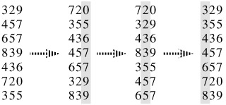
Radix sort solves the sorting problem counterintuitively - by sorting on the least significant digit first. In order for it to work, the digit sorts must be stable. The code for radix sort is straightforward. The following procedure assumes that each element in the n-element array A has d digits, where digit 1 is the lowest-order digit and digit d is the highest-order digit.
RADIX-SORT(A,d)
for i = 1 to d
	use a stable sort to sort array A on digit i
Is radix sort preferable to a comparison-based sorting algorithm, such as quicksort? Which sorting algorithm we prefer depends on the characteristics of the implementations, of the underlying machine (e.g., quicksort often uses hardware caches more effectively than radix sort), and of the input data. Moreover, the version of radix sort that uses counting sort as the intermediate stable sort does not sort in place, which many of the Θ(nlgn)-time comparison sorts do. Thus, when primary memory storage is at a premium, we might prefer an in-place algorithm such as quicksort.
Bucket sort
Bucket sort assumes that the input is drawn from a uniform distribution and has an average-case running time of O(n). Like counting sort, bucket sort is fast because it assumes something about the input. Whereas counting sort assumes that the input consists of integers in a small range, bucket sort assumes that the input is generated by a random process that distributes elements uniformly and independently over the interval [0,1).
Bucket sort divides this interval into n equal-size subintervals, or buckets, and then distributes the n input numbers into the buckets. Since the inputs are uniformly and independently distributed, we don’t expect many numbers to fall into each bucket. To produce the output, we simply sort the numbers in each bucket and then go through the buckets in order, listing the elements in each.
BUCKET-SORT(A)
n = A.length
let B[0..n - 1] be a new array
for i = 0 to n - 1
	make B[i] an empty list
for i = 1 to n
	insert A[i] into list B[floor(n*A[i])]
for i = 0 to n - 1
	sort list B[i] with insertion sort
concat the lists B[0], B[1], ..., B[n - 1] together in order
Even if the input is not drawn from a uniform distribution, bucket sort may still run in linear time. As long as the input has the property that the sum of the squares of the bucket sizes is linear in the total number of elements, the bucket sort will run in linear time.